Git beyond Commits, and Pulling-Pushing
Git does extreamely complicated things in simple ways. Let’s jump right in.
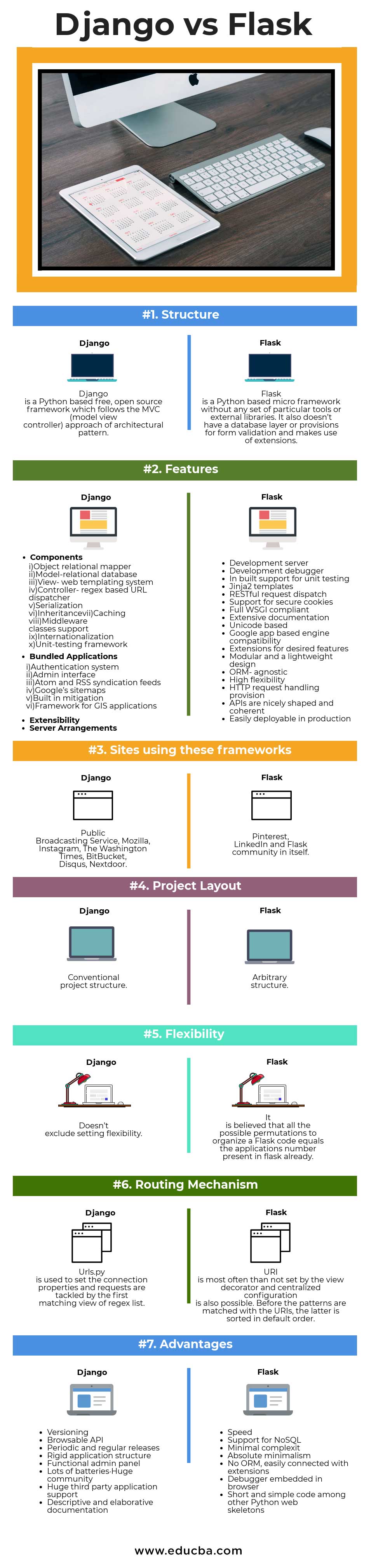
Django vs Flask in the context of Deploying ML/AI
Django and Flask are both frameworks for creating web applications in Python. Django provides a full-featured MVC Framework that includes the whole kitchen sink. While Django alone could be used to make a RESTful API, Django REST Framework is a fantastic, feature-filled extension to the Django framework.
Flask is a micro-framework that follows the Unix philosophy of “do one thing and do it well”. Flask provides very little upfront, not even an ORM, but the community provides a large set of extensions that match a lot of Django’s feature set.
A popular idiom to compare the two frameworks is that ‘Pirates use Flask, The Navy uses Django.‘
What They Have In Common
While Django and Flask take different approaches to designing a web platform, they support a lot of the same capabilities when it comes to REST API design. This analysis assumes Django is using the Django REST Framework toolkit, and Flask is using various popular plugins necessary to achieve comparable results.
User Auth
Django REST Framework supports using Django’s built-in user model for API authentication and authorization (docs). With Flask, you can use built-in tools for basic auth, or third-party plugin such as Flask-HTTPAuth for more complex scenarios. Miquel Grinberg provides a thorough tutorial for creating API endpoints using Flask-HTTPAuth.
Rate Limiting
Django REST framework supports throttling of both anonymous and registered users (docs). Flask, along with the Flask-Limiter plugin, support a similar feature set. Both platforms support in-memory, Memcached, or Redis backends for store rate limitation data.
Relational Database Mapping
Django REST Framework provides a straightforward method of mapping Django ORM models to API endpoints (docs). Flask, along with Flask-Restless, provides similar capabilities for an SQLAlchemy database model (docs). Both frameworks provide a simple path to creating a CRUD interface for an existing data store.
Advantages of Django with Django REST Framework
Versioning
Handling multiple versions of an API is never a simple endeavor. Django REST Framework includes support for versioning is fairly flexible, making the task a little less onerous. The toolkit supports multiple URL formats (example.com/v1/sample/, v1.example.com/sample/, or example.com/sample/?version=v1), and the version is passed in as a request parameter (request.version) to be used in a view.
Versioning can be handled in Flask, but it has to be managed by the developers. In fact, many solutions involve structuring the entire hierarchy of the application to support the concept of versioning.
Browsable API
Django REST Framework generates HTML pages to browse and execute all API endpoints. With this feature, users and/or developers can execute GETs and POSTs quickly and easily in their browser. Even if disabled for production use, this is a fantastic feature for testing and demos.
Flask does not have a good Browseable API option. The creator of Django REST Framework created a similar library for Flask called Flask-API, but it is not under active development nor is it ready for production use. Another option is to use the swagger API wrapper in front of the API, but maintaining the swagger schema would take time.
Regular Releases
Django and Django REST Framework are both under heavy active development. Django has a major release twice per year with an LTS release every two years. Django REST Framework has had three major releases in the last year. Flask, on the other hand, last had a tagged release in 2013. This does not mean the project is dead, as the multitude of plugin libraries receive regular updates, but the contrast with Django is noteworthy.
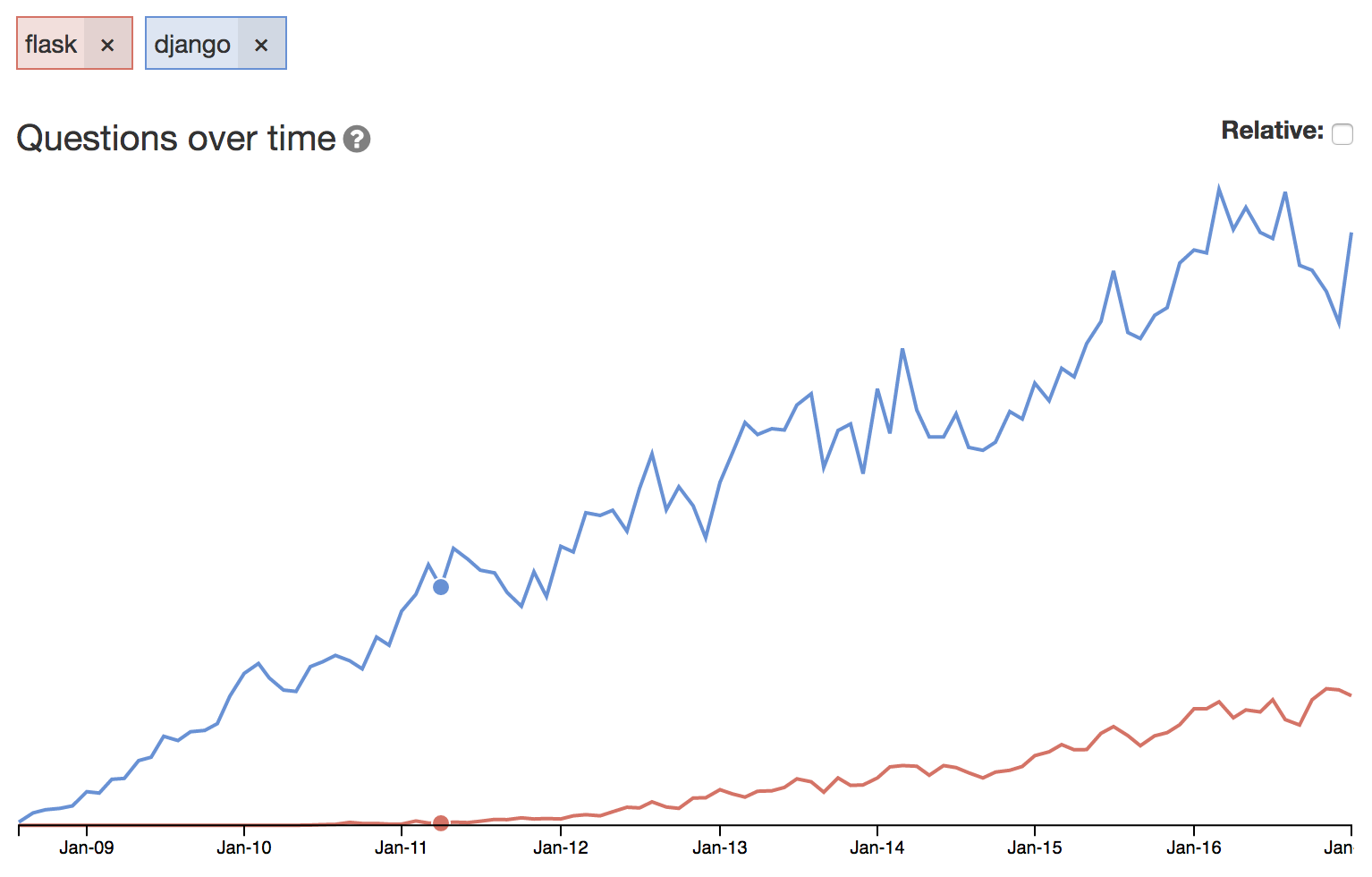
##Community Help
This is a graph of total questions asked on Django/Flask in stackoverflow.
Advantages of Flask
Speed
Flask is able to achieve generally faster performance than Django(without any specific enhancements, Django can also be customized for handling multiple requests and efficiency), generally due to the fact that Flask is much more minimal in design. While both of these frameworks can support several hundred queries per second without breaking a sweat, neither were designed with a priority on speed(As our application focuses mostly on DL, there will be fewer requests but the requests themselves will be computationally expensive, so this does not hold that much). Falcon and Bottle are Python web frameworks that emphasize speed, albeit with much smaller developer communities, and are worth a look if speed is more important than support and features.
NoSQL Support (Not a major thing)
The Django platform heavily ties itself to relational database integration. An extension called django-rest-framework-mongoengine wires Mongo into Django REST Framework, but I can’t speak for its ease of use. Because Flask has no built-in ORM, it is more freely able to integrate with NoSQL databases like MongoDB (via mongokit or Flask-Pymongo) and DynamoDB (via Flask-Dynamo). In addition, the Eve toolkit, a wrapper on top of Flask, includes built-in support for MongoDB.
Instagram, Disqus, Bitbucket, Websites of Onion, Firefox, NASA, The Washington Post use Django.
While Pinterest uses Flask.
Personal Experience
Django has a far steeper learning curve than Flask and is more complex and intricate, but in the long run, it has the flexibilities to scale with more users/intricate features. Flask is far easier to start (You could go from zero knowledge on flask to deploying a DL model on Flask for some specific case, i.e. a finished end product, in about a week of hard work), especially it’s easier to host and serve. But even if Django is harder, it has loads of flexibility and has a very strong community support, having loads of apps built onto it for specific use cases (like django-imagekit for example, the GitHub repo mentioned in the mail).
Why Tensorflow, why not PyTorch?
Useful Links
These are some helpful links for further research. These post is a compilation of all these resources and my own experience.
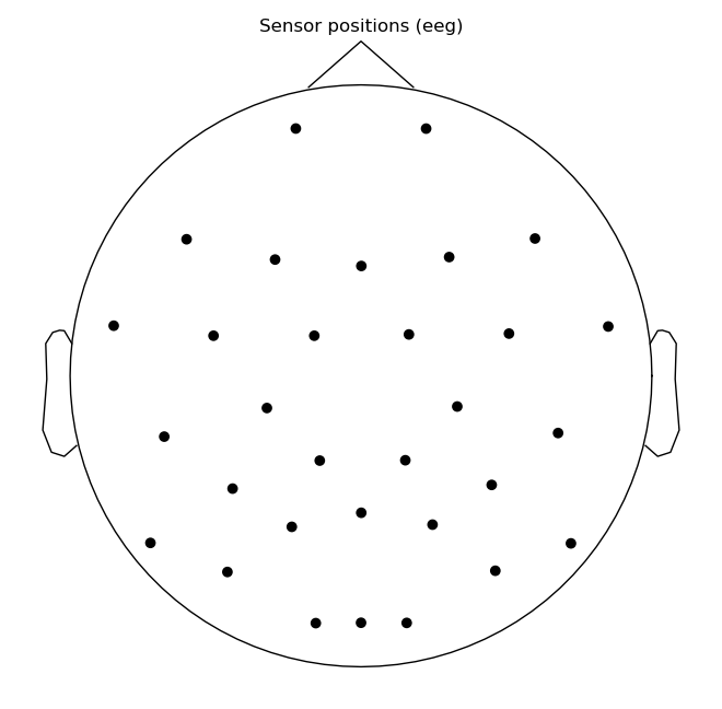
Basic EEG Processing with MNE
A very basic pipeline of processing EEG data Offline, using MNE-Python.
%matplotlib qt
import mne
import numpy as np
import os.path as op
from matplotlib import pyplot as plt
from mne import Epochs, pick_types, events_from_annotations
from mne.preprocessing import ICA
from mne.preprocessing import create_eog_epochs, create_ecg_epochs
from mne.channels import read_layout
from mne.io import concatenate_raws, read_raw_edf
from mne.decoding import CSP

from sklearn.pipeline import Pipeline
from sklearn.discriminant_analysis import LinearDiscriminantAnalysis
from sklearn.model_selection import ShuffleSplit, cross_val_score

print(__doc__)
Automatically created module for IPython interactive environment
# Data Folder Path
data_path = 'EEG_data'

# Specific File Name Appending
fname = data_path + '\AC32-000003-7s-handmov-4ch.vhdr'

raw = mne.io.read_raw_brainvision(fname,preload=True)
Extracting parameters from EEG_data\AC32-000003-7s-handmov-4ch.vhdr...
Setting channel info structure...
Reading 0 ... 197649  =      0.000 ...   395.298 secs...
raw.info
<Info | 16 non-empty fields
    bads : list | 0 items
    ch_names : list | Fp1, Fz, F3, F7, FT9, FC5, FC1, C3, T7, ...
    chs : list | 31 items (EEG: 31)
    comps : list | 0 items
    custom_ref_applied : bool | False
    dev_head_t : Transform | 3 items
    events : list | 0 items
    highpass : float | 0.0 Hz
    hpi_meas : list | 0 items
    hpi_results : list | 0 items
    lowpass : float | 140.0 Hz
    meas_date : tuple | 2019-06-14 15:33:55 GMT
    nchan : int | 31
    proc_history : list | 0 items
    projs : list | 0 items
    sfreq : float | 500.0 Hz
    acq_pars : NoneType
    acq_stim : NoneType
    ctf_head_t : NoneType
    description : NoneType
    dev_ctf_t : NoneType
    dig : NoneType
    experimenter : NoneType
    file_id : NoneType
    gantry_angle : NoneType
    hpi_subsystem : NoneType
    kit_system_id : NoneType
    line_freq : NoneType
    meas_id : NoneType
    proj_id : NoneType
    proj_name : NoneType
    subject_info : NoneType
    xplotter_layout : NoneType
>
montage = mne.channels.read_montage('standard_1020')
print(montage)
<Montage | standard_1020 - 97 channels: LPA, RPA, Nz ...>
raw.set_montage(montage,set_dig=True,verbose=True)
<RawBrainVision | AC32-000003-7s-handmov-4ch.eeg, n_channels x n_times : 31 x 197650 (395.3 sec), ~46.8 MB, data loaded>
raw.plot_sensors()
raw.ch_names
['Fp1',
 'Fz',
 'F3',
 'F7',
 'FT9',
 'FC5',
 'FC1',
 'C3',
 'T7',
 'TP9',
 'CP5',
 'CP1',
 'Pz',
 'P3',
 'P7',
 'O1',
 'Oz',
 'O2',
 'P4',
 'P8',
 'TP10',
 'CP6',
 'CP2',
 'C4',
 'T8',
 'FT10',
 'FC6',
 'FC2',
 'F4',
 'F8',
 'Fp2']
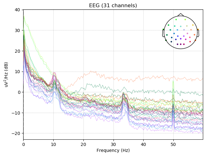
raw.plot_psd(fmax=60)
Effective window size : 4.096 (s)
np.shape(raw._data)
(31, 197650)
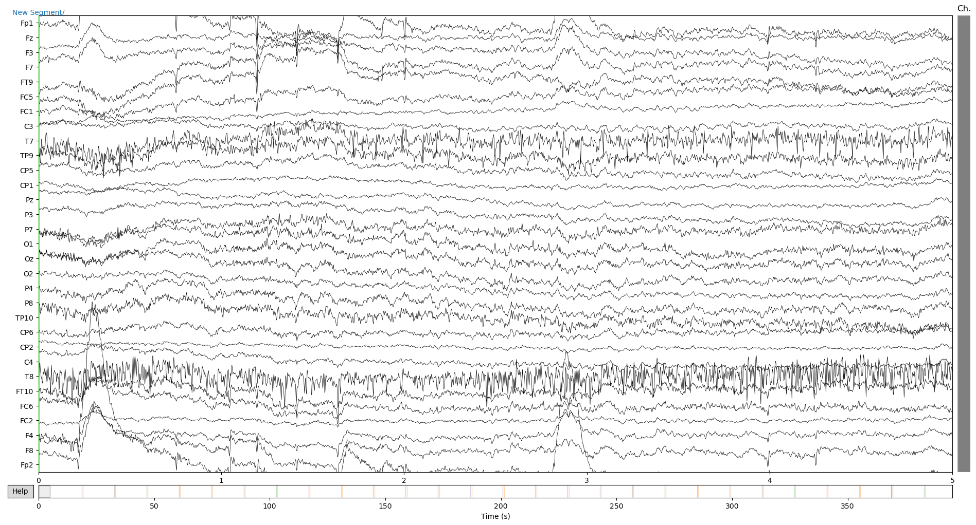
raw.plot(duration=5, n_channels=31)
picks = pick_types(raw.info, meg=False, eeg=True, stim=False, eog=False,
exclude='bads')
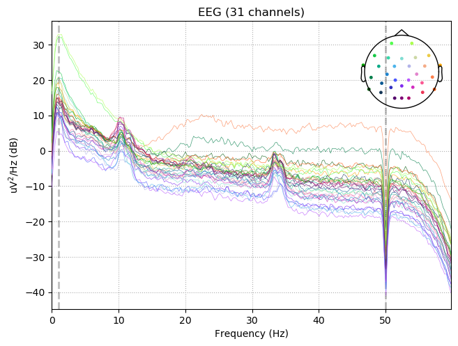
raw.notch_filter(np.arange(50, 201, 50), picks=picks, fir_design='firwin')
raw.filter(1,50., None, n_jobs=1, fir_design='firwin')
raw.plot_psd(tmax=np.inf, fmax=60)
Setting up band-stop filter

FIR filter parameters
---------------------
Designing a one-pass, zero-phase, non-causal bandstop filter:
- Windowed time-domain design (firwin) method
- Hamming window with 0.0194 passband ripple and 53 dB stopband attenuation
- Lower transition bandwidth: 0.50 Hz
- Upper transition bandwidth: 0.50 Hz
- Filter length: 3301 samples (6.602 sec)

Filtering raw data in 1 contiguous segment
Setting up band-pass filter from 1 - 50 Hz

FIR filter parameters
---------------------
Designing a one-pass, zero-phase, non-causal bandpass filter:
- Windowed time-domain design (firwin) method
- Hamming window with 0.0194 passband ripple and 53 dB stopband attenuation
- Lower passband edge: 1.00
- Lower transition bandwidth: 1.00 Hz (-6 dB cutoff frequency: 0.50 Hz)
- Upper passband edge: 50.00 Hz
- Upper transition bandwidth: 12.50 Hz (-6 dB cutoff frequency: 56.25 Hz)
- Filter length: 1651 samples (3.302 sec)

Effective window size : 4.096 (s)
method = 'fastica'
n_components = 25
random_state = 23
ica = ICA(n_components=n_components, method=method, random_state=random_state)
print(ica)
<ICA | no decomposition, fit (fastica): samples, no dimension reduction>
ica.fit(raw)
print(ica)
Fitting ICA to data using 31 channels (please be patient, this may take a while)
Inferring max_pca_components from picks
Selection by number: 25 components
Fitting ICA took 7.0s.
<ICA  |  raw data decomposition, fit (fastica): 197650 samples, 25 components, channels used: "eeg">
ica.plot_components(inst=raw, psd_args={'fmax': 35.})
[<Figure size 750x700 with 20 Axes>, <Figure size 750x250 with 5 Axes>]
# Include the channels which are Bad (BE CAREFUL not to exclude Real Features in Data useful for classification)
eog_inds = [0,1,2]
ica.exclude.extend(eog_inds)
raw_copy = raw.copy()
ica.apply(raw_copy)
Transforming to ICA space (25 components)
Zeroing out 3 ICA components


<RawBrainVision  |  AC32-000003-7s-handmov-4ch.eeg, n_channels x n_times : 31 x 197650 (395.3 sec), ~46.8 MB, data loaded>
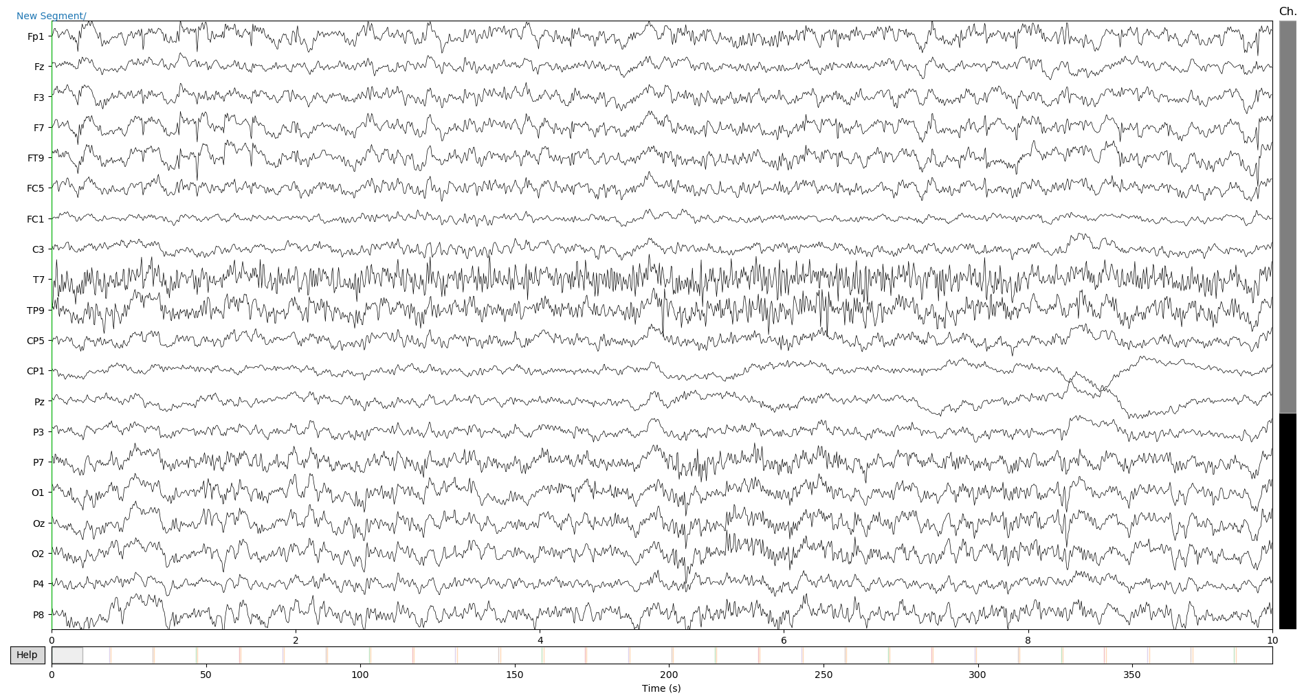
raw_copy.plot()
annot = raw.annotations
annot[1]
OrderedDict([('onset', 18.684),
             ('duration', 0.002),
             ('description', 'Stimulus/S 20'),
             ('orig_time', 1560526435.391673)])
annot[7]['onset']-annot[5]['onset']
14.012
raw_copy.annotations
<Annotations | 55 segments : New Segment/ (1), Stimulus/S 20 (7), Stimulus/S 16 (27)..., orig_time : 2019-06-14 15:33:55.391673>
events, _ = mne.events_from_annotations(raw)
Used Annotations descriptions: ['New Segment/', 'Stimulus/S 16', 'Stimulus/S 17', 'Stimulus/S 18', 'Stimulus/S 20', 'Stimulus/S 24']
type(events)
numpy.ndarray
events
array([[     0,      0,  99999],
       [  9342,      0,     20],
       [  9592,      0,     16],
       [ 16356,      0,     24],
       [ 16606,      0,     16],
       [ 23357,      0,     17],
       [ 23607,      0,     16],
       [ 30363,      0,     18],
       [ 30613,      0,     16],
       [ 37378,      0,     20],
       [ 37628,      0,     16],
       [ 44383,      0,     24],
       [ 44634,      0,     16],
       [ 51389,      0,     17],
       [ 51639,      0,     16],
       [ 58389,      0,     18],
       [ 58639,      0,     16],
       [ 65394,      0,     20],
       [ 65644,      0,     16],
       [ 72394,      0,     24],
       [ 72645,      0,     16],
       [ 79394,      0,     17],
       [ 79644,      0,     16],
       [ 86399,      0,     18],
       [ 86650,      0,     16],
       [ 93409,      0,     20],
       [ 93659,      0,     16],
       [100417,      0,     24],
       [100667,      0,     16],
       [107430,      0,     17],
       [107680,      0,     16],
       [114434,      0,     18],
       [114684,      0,     16],
       [121435,      0,     20],
       [121685,      0,     16],
       [128444,      0,     24],
       [128695,      0,     16],
       [135452,      0,     17],
       [135702,      0,     16],
       [142450,      0,     18],
       [142700,      0,     16],
       [149454,      0,     20],
       [149704,      0,     16],
       [156455,      0,     24],
       [156705,      0,     16],
       [163453,      0,     17],
       [163703,      0,     16],
       [170453,      0,     18],
       [170703,      0,     16],
       [177455,      0,     20],
       [177705,      0,     16],
       [184451,      0,     24],
       [184701,      0,     16],
       [191465,      0,     17],
       [191715,      0,     16]])
events_new = events[1::2,:]
# As 4 events are there in sequential manner
events_new[0::4,2] = 1
events_new[1::4,2] = 2
events_new[2::4,2] = 3
events_new[3::4,2] = 4
events_new
array([[  9342,      0,      1],
       [ 16356,      0,      2],
       [ 23357,      0,      3],
       [ 30363,      0,      4],
       [ 37378,      0,      1],
       [ 44383,      0,      2],
       [ 51389,      0,      3],
       [ 58389,      0,      4],
       [ 65394,      0,      1],
       [ 72394,      0,      2],
       [ 79394,      0,      3],
       [ 86399,      0,      4],
       [ 93409,      0,      1],
       [100417,      0,      2],
       [107430,      0,      3],
       [114434,      0,      4],
       [121435,      0,      1],
       [128444,      0,      2],
       [135452,      0,      3],
       [142450,      0,      4],
       [149454,      0,      1],
       [156455,      0,      2],
       [163453,      0,      3],
       [170453,      0,      4],
       [177455,      0,      1],
       [184451,      0,      2],
       [191465,      0,      3]])
# Starting the epochs 1 second before stim onset and ending 7 s after onset
# But will crop later to avoid classification of evoked responses by using epochs that start 1s after stim onset
tmin, tmax = -1., 6.

# Giving proper labels to the events
event_id = {'Left': 1, 'Right': 2, 'Up': 3, 'Down': 4}

picks = pick_types(raw_copy.info, meg=False, eeg=True, stim=False, eog=False,
                   exclude='bads')

epochs = mne.Epochs(raw_copy, events_new, event_id, tmin, tmax, picks=picks,
                baseline=None, preload=True)
27 matching events found
No baseline correction applied
Not setting metadata
0 projection items activated
Loading data for 27 events and 3501 original time points ...
0 bad epochs dropped
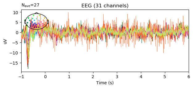
epochs.average().plot(spatial_colors=True, time_unit='s')
color = {1: 'green', 2: 'yellow', 3: 'red', 4: 'black'}

mne.viz.plot_events(events_new, raw.info['sfreq'], raw.first_samp, color=color,
                    event_id=event_id)
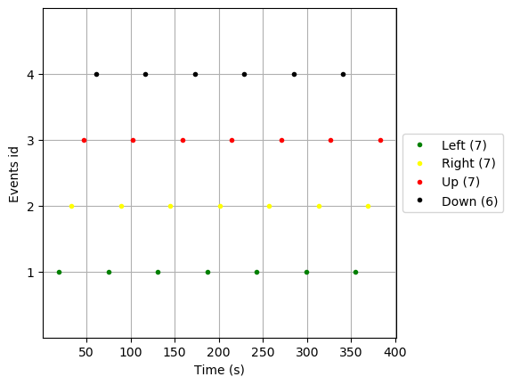
print(epochs['Left'])
print(epochs.event_id)
print(epochs.events)
<Epochs  |   7 events (all good), -1 - 6 sec, baseline off, ~5.9 MB, data loaded,
 'Left': 7>
{'Left': 1, 'Right': 2, 'Up': 3, 'Down': 4}
[[  9342      0      1]
 [ 16356      0      2]
 [ 23357      0      3]
 [ 30363      0      4]
 [ 37378      0      1]
 [ 44383      0      2]
 [ 51389      0      3]
 [ 58389      0      4]
 [ 65394      0      1]
 [ 72394      0      2]
 [ 79394      0      3]
 [ 86399      0      4]
 [ 93409      0      1]
 [100417      0      2]
 [107430      0      3]
 [114434      0      4]
 [121435      0      1]
 [128444      0      2]
 [135452      0      3]
 [142450      0      4]
 [149454      0      1]
 [156455      0      2]
 [163453      0      3]
 [170453      0      4]
 [177455      0      1]
 [184451      0      2]
 [191465      0      3]]
# Check Visualization here
ev_left = epochs['Left'].average()
ev_right = epochs['Right'].average()
ev_up = epochs['Up'].average()
ev_down = epochs['Down'].average()

f, axs = plt.subplots(2 , 2, figsize=(10, 5))
_ = f.suptitle('Left Right Up Down Hand Movement Imagine', fontsize=20)
_ = ev_left.plot(axes=axs[0, 0], show=False, time_unit='s')
_ = ev_right.plot(axes=axs[0 ,1], show=False, time_unit='s')
_ = ev_up.plot(axes=axs[1, 0], show=False, time_unit='s')
_ = ev_down.plot(axes=axs[1, 1], show=False, time_unit='s')
plt.tight_layout()
epoch3d = epochs.get_data()
np.shape(epoch3d)
(27, 31, 3501)
epochs.plot_image()
27 matching events found
No baseline correction applied
Not setting metadata
0 projection items activated
0 bad epochs dropped


[<Figure size 640x480 with 3 Axes>]
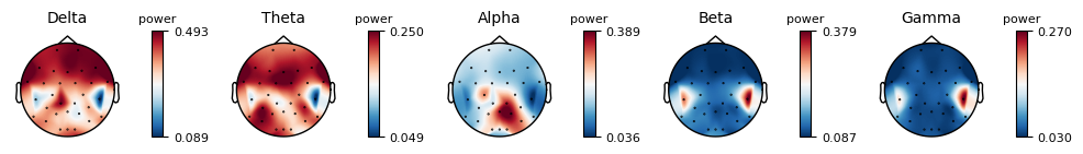
epochs.plot_psd_topomap( normalize=True)
Using multitaper spectrum estimation with 7 DPSS windows
from mne.time_frequency import tfr_morlet, psd_multitaper

l_epochs = epochs['Left']
r_epochs = epochs['Right']
u_epochs = epochs['Up']
d_epochs = epochs['Down']


freqs = np.logspace(*np.log10([6, 35]), num=8)
n_cycles = freqs / 2.  # different number of cycle per frequency

power,itc = tfr_morlet(epochs, freqs=freqs, n_cycles=n_cycles, use_fft=True,
                        return_itc=True, n_jobs=4)

l_power, l_itc = tfr_morlet(l_epochs, freqs=freqs, n_cycles=n_cycles, use_fft=True,
                        return_itc=True, n_jobs=4)
r_power, r_itc = tfr_morlet(r_epochs, freqs=freqs, n_cycles=n_cycles, use_fft=True,
                        return_itc=True, n_jobs=4)
u_power, u_itc = tfr_morlet(u_epochs, freqs=freqs, n_cycles=n_cycles, use_fft=True,
                        return_itc=True, n_jobs=4)
d_power, d_itc = tfr_morlet(d_epochs, freqs=freqs, n_cycles=n_cycles, use_fft=True,
                        return_itc=True, n_jobs=4)
[Parallel(n_jobs=4)]: Using backend LokyBackend with 4 concurrent workers.
[Parallel(n_jobs=4)]: Done  14 tasks      | elapsed:    0.8s
[Parallel(n_jobs=4)]: Done  31 out of  31 | elapsed:    1.3s finished
[Parallel(n_jobs=4)]: Using backend LokyBackend with 4 concurrent workers.
[Parallel(n_jobs=4)]: Done   7 out of  31 | elapsed:    0.0s remaining:    0.2s
[Parallel(n_jobs=4)]: Done  31 out of  31 | elapsed:    0.3s finished
[Parallel(n_jobs=4)]: Using backend LokyBackend with 4 concurrent workers.
[Parallel(n_jobs=4)]: Done   7 out of  31 | elapsed:    0.0s remaining:    0.2s
[Parallel(n_jobs=4)]: Done  31 out of  31 | elapsed:    0.4s finished
[Parallel(n_jobs=4)]: Using backend LokyBackend with 4 concurrent workers.
[Parallel(n_jobs=4)]: Done   7 out of  31 | elapsed:    0.0s remaining:    0.3s
[Parallel(n_jobs=4)]: Done  31 out of  31 | elapsed:    0.4s finished
[Parallel(n_jobs=4)]: Using backend LokyBackend with 4 concurrent workers.
[Parallel(n_jobs=4)]: Done   7 out of  31 | elapsed:    0.0s remaining:    0.3s
[Parallel(n_jobs=4)]: Done  31 out of  31 | elapsed:    0.3s finished
u_power.plot_topo(baseline=(-0.5, 0), mode='logratio', title='Average power')
u_power.plot([26], baseline=(-0.5, 0), mode='logratio', title=power.ch_names[26])

fig, axis = plt.subplots(1, 2, figsize=(7, 4))
u_power.plot_topomap(ch_type='eeg', tmin=0.5, tmax=1.5, fmin=8, fmax=12,
                   baseline=(-0.5, 0), mode='logratio', axes=axis[0],
                   title='Down Alpha', show=False)
u_power.plot_topomap(ch_type='eeg', tmin=0.5, tmax=1.5, fmin=13, fmax=25,
                   baseline=(-0.5, 0), mode='logratio', axes=axis[1],
                   title='Down Beta', show=False)
mne.viz.tight_layout()
plt.show()
Applying baseline correction (mode: logratio)
Applying baseline correction (mode: logratio)
Applying baseline correction (mode: logratio)
Applying baseline correction (mode: logratio)
power_data = u_power.data
np.shape(power_data)
(31, 8, 3501)
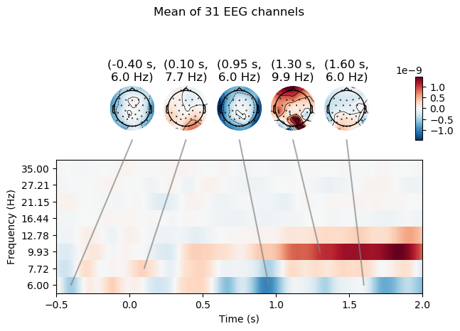
power.plot_joint(baseline=(-0.5, 0), mode='mean', tmin=-.5, tmax=2,
                 timefreqs=[(.95, 6), (1.3, 9.5), (-0.4, 6), (0.1, 7.7), (1.6, 6.0)])
Applying baseline correction (mode: mean)
Applying baseline correction (mode: mean)
Applying baseline correction (mode: mean)
Applying baseline correction (mode: mean)
Applying baseline correction (mode: mean)
Applying baseline correction (mode: mean)
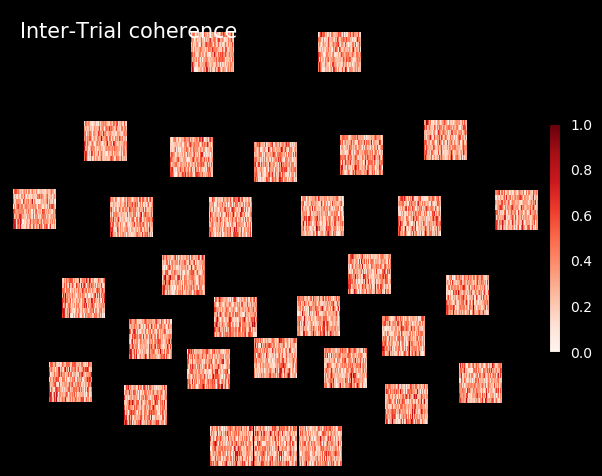
r_itc.plot_topo(title='Inter-Trial coherence', vmin=0., vmax=1., cmap='Reds')
No baseline correction applied
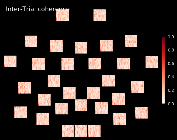
itc.plot_topo(title='Inter-Trial coherence', vmin=0., vmax=1., cmap='Reds')
No baseline correction applied
raw_copy.save('postica_ayan7shandmov4ch-raw.fif',
         overwrite=True)
Writing C:\Users\Nal\Desktop\bciayan\postica_ayan7shandmov4ch-raw.fif
Closing C:\Users\Nal\Desktop\bciayan\postica_ayan7shandmov4ch-raw.fif [done]
epochs.save('epochs-ayan7shandmov4ch-epo.fif',
         overwrite=True)
You Should Start Doing Kaggle. Now. Period.
Say you’ve heard the terms Data Science/Machine Learning somewhere quite sometime ago. You are genuinely interested in that work, you’ve started some MOOC’s, played with some datasets, have a small project. Now, what’s next? What’s best for you?
It’s surprising that even though you maybe interested in completely different applications, unique career paths, but still Kaggle is the best answer for nearly all of them. It’s currently the best way to learn, test your skills, and get your hands dirty in the truest sense.
So whatever you know about Data Science, if you wish to do better than you are doing, you should be spending more time in Kaggle.
Index To OpenSource Contributions
This page acts as an index to all my contributions in terms of Pull Requests to Open Source Organizations.
AboutCode
-
Adds Travis-CI for sphinx-build and linkcheck
This adds test scripts to check build status of Spinx Documentation along with adding checks for broken links. Also fixes some broken links and updates doc_maintenance.rst
-
Adds Documentation from Wiki
To the main documentation this adds Deltacode, Aboutcode Docs and remaining pages of ScanCode Toolkit and ScanCode Workbench from wiki.
-
Adds GitHub wiki of Scancode-Toolkit and Scancode-Workbench
This adds almost all the Wiki Pages of Scancode-Toolkit (Except the How-To pages) and Scancode-Workbench.
Index To Neuroscience Blogs
I’ve just started chasing my dreams of knowing how the Brain works, and here I document my experiences, opinions, materials that I compiled and hope that it’ll be useful for others, book reviews, tutorials on EEG processing related topics and more!
This page acts as an index to all my Neuroscience related blog posts. Cheers!
Blogs
Other Resources
Index To Kaggle Club Blogs and Public Kernels
This page acts as an index to all my Kaggle Kernels, Kaggle competetions I’ve participated in, and everything related to the University Kaggle Club. Cheers!
Kaggle Kernels
Kaggle Competetions
-
Top 41%. 867th out of 2131 Participants